Conjoint Analysis – ten years later
We are often asked why a company that specializes in consulting operations management is called Data Assessment Solutions. The answer to this question today still determines the direction in which we at DAS Research think. Even before DAS was founded, it was clear to us that many questions could not be answered only with the help of data from passive data, that is, data that was not explicitly collected to answer the question. Data must therefore also be collected actively in a data assessment. A very important example for us are employee skills, which we initially collected completely in a skills assessment. Today, we can also learn skills from passive sources such as CVs and project histories. To ensure a good data quality, we are still actively collecting skills data, albeit on a much smaller scale. Another topic that we tackled ten years ago is the measurement of preferences. To collect and evaluate preference data for our IT Skills Study 2009, we have developed methods for carrying out and evaluating conjoint analysis studies. In this article we explain how we reduced the evaluation of the conjoint analysis studies with a geometric trick to a standard problem of machine learning.
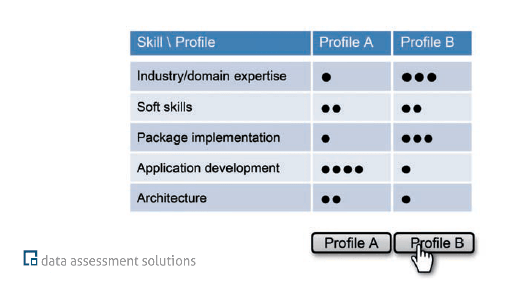
In a conjoint analysis, objects that are described by several attributes are compared with each other. In our case, the objects were IT profiles comprised of five IT skills. An IT profile is defined by a competency level, on a five-level scale, for each of the five IT skills. The study participants were shown twelve randomly generated pairs of IT profiles, one after the other. They were asked to select the profile of the candidate they would rather hire. From the paired comparisons, we then learned a partworth value for each competence level for each of the five IT skills, i.e. a total of 25 partworth values. With the help of the partworth values we were able to say which skills are more and which are less important and for which skills an improvement of the competence level pays off the most.
The calculation of the partworth values was reduced to a binary classification problem by a simple trick: We identified each paired comparison with a hyperplane in 25-dimensional space, that is we divided the 25-dimensional space linearly into two halves, the half space above the hyperplane and the half space below it. The answer to a paired comparison indicates whether the vector of the 25 partworth values is above or below the hyperplane. At the end, we look for a partworth vector that lies in the intersection of all the half spaces given by the paired comparisons. If the section is empty, we look for a partworth vector that violates the geometric conditions given by the paired comparisons as little as possible. Thus, the data given by the paired comparisons are interpreted as hyperplanes labeled either above (+1) or below (-1) depending on the outcome of the comparison, and we are looking for a vector (point in 25-dimensional space) that is compatible with this data.
The situation is surprisingly like a linear binary classification problem. The data here are binary (-/+ 1)-labelled points, and we are looking for a hyperplane that divides the space in a way that on each side of the plane only points with a label can be found, if possible. The solution of such problems is a standard task in machine learning and is solved among others by support vector machines (SVMs) or by logistic regression. The difference to our conjoint analysis problem is that in the first case the data are labeled hyperplanes and a compatible point needs to be computed, whereas in the second case the data are labeled points and a compatible hyperplane needs to be computed.
In geometry, points and hyperplanes are dual to each other, that is, points can also be interpreted as hyperplanes and hyperplanes as points. The idea behind this is very easy to understand in two-dimensional Euclidean space. A point in two-dimensional space is described by two coordinates (x- and y-coordinate). A hyperplane in two-dimensional space is simply a straight line, which is also described by two coordinates: the y-axis section and the slope of the straight line. In a duality theory, only the pairs of coordinates are considered and either interpreted as a point or as a hyperplane. In Euclidean geometry, however, there are cases in which the reinterpretation does not work. Unfortunately, these so-called singular cases occur in our conjoint analysis problem. For some of the labeled hyperplanes there is no dual point. If Euclidean geometry is extended to the projective geometry by adding points and a hyperplane at infinity, the singular cases disappear. The labelled hyperplanes, which are problematic in our conjoint analysis setting, are dual to points at infinity. In projective geometry one can continue to calculate with these points without any problems.
In the evaluation of our Skills study, we simply translated the conjoint analysis problem into a linear binary classification problem by using projective duality. He latter problem was easily solved with a standard support vector machine software.